Basic Rules of Probability

\(P(A), P(B), …\) represents probability of occurrence of events \(A, B, …\)

Probability of any event \(X\) can be calculated as the ratio of the number of chances favorable for event \(X\) to the total number of chances:

i.e.; \(P(X) = \frac{m_X}{n}\)

where, \(n\) is the total number of chances & \(m_X\) is the number of chances favorable for event \(X\)

Probability of any random event lies between \(0\) & \(1\)

i.e.;  \(0 \leq P(X) \leq 1\)

Event \(X\) is called practically sure if its probability is not exactly but very close to \(1\)

i.e.; \(P(X) \approx 1\)

Event \(X\) is called practically impossible if its probability is not exactly but very close to \(0\)

i.e.; \(P(X) \approx 0\)

Probability summation rule

The Probability that one of two (or more) mutually exclusive events occurs is equal to the sum of the Probabilities of these events

i.e.; \(P(X or Y) = P(X) + P(Y)\)

if events \(X_1, X_2, …, X_n \) are mutually exclusive and exhaustive, the sum of their Probabilities is equal to \(1\)

i.e.; \(P(X_1) + P(X_2) + … + P(X_n) = 1\)

From the above statement it follows that Probability of an event \(X\) and its opposite(non occurrence) i.e.; \( !X\), is equal to \(1\)

i.e.; \(P(X) + P(!X) =1\)

Probability multiplication rule

The Probability of the combination of  two  events (simultaneous occurrence) is equal to the Probability of one of them multiplied by the probability of the other provided that the first event has occured.

i.e.; \(P(A and B) = P(A, B) = P(A) P(B | A)\)

where \(P(B | A)\) is called conditional probability of an event \(B\) calculated for the condition that event \(A\) has occurred.

Event sets used in examples section

Event Set 1

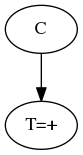
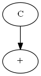
\(C\): Event of the occurrence of a specific type of Cancer

\(P(C)\): Probability of occurrence of event C.

\(P(!C) = 1- P(C)\)

\((T = +)\): Event that a test is positive for C. (Sometimes we will represent it with just a \(+\))

\(P(T = -) = 1 -P(T = +)\) OR \(P(-) = 1- P(+)\)

Event Set 2

\(S\): Event that the weather is Sunny.

\(R\): Event that the person gets a raise.

\(H\): Event that the person is happy.

 

Bayes’ Theorem

   

 

\(P(C | +) = \frac{P(C) P(+ | C)}{P(+)} = \frac{P(C) P(+ | C)}{P(C) P(+ |C) + P(!C) P(+ | !C)}\)

where:-

\(P(C | +)\): is Posterior

\(P(+ | C)\): is Likelihood

\(P(C)\): is Prior

\(P(+)\): Marginal Likelihood

Bayes’ Theorem gives us a framework to modify our beliefs in light of new evidences. Bayesian statistics gives us a solid mathematical means of incorporating our prior beliefs and evidence, to produce new posterior beliefs.

(NOTE: I will expand upon this in some future blog post).

 

Causal Graph

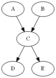
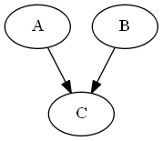
Causal Graphs  (also called Causal Bayesian Networks) are directed acyclic graphs which are used to encode assumptions about the Probabilistic data represented by variables.

For example in the above graph, joint Probability represented by Bayes’ Network is given by:

\(P(A, B, C, D, E) = P(A) P(B) P(C | A, B) P(D | C) P(E | C)\)

This example requires 10 values to represent the network. These are:

1. \(P(A)\)
2. \(P(B)\)
3. \(P(C | A, B)\)
4. \(P(C | !A, B)\)
5. \(P(C | A, !B)\)
6. \(P(C | !A, !B)\)
7. \(P(D | C)\)
8. \(P(D | !C)\)
9. \(P(E | C)\)
10. \(P(E | !C)\)

 

D-Separation

D-separation is a criterion for deciding, from a given causal graph, whether a variable (OR set of variables) \(X\) is independent of another variable (OR set of variables) \(Y\), given a third variable (OR set of variables) \(Z\). This has to do with path or reachability.

So when we think in terms of types of D-Separation we need to further break it down in terms of Active or Inactive triplets.

(NOTE: In listed types, I have highlighted node(s) in gray color to show involvement.)

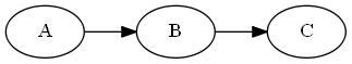
Type 1 (causal chain)

Active Triplets :

Given that \(B\) is involved, \(A\) & \(C\) are independent.

i.e.; \(P(C | B, A) = P(C | B)\)

Inactive Triplets

Given that \(B\) is not involved, \(A\) & \(C\) are dependent

i.e.; \(P(C | A) eq P(C)\)

 

Type 2 (common cause)

Active Triplets (Conditional Independence)

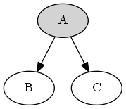
Given that \(A\) is involved, \(B\) & \(C\) become independent (Conditional independence) .

i.e.; \(P(C | A, B) = P(C | A) \)

Remember, Conditional Independence does not guarantee absolute independence

i.e.; \(P(C | B) = P(C | B, A) P( A | B) = P(C | A) P(A | B)\)

Inactive Triplets

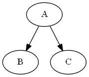
Given that \(A\) is not involved, \(B\) & \(C\) become dependent.

i.e.; \(P(C | B) eq P(C)\)

 

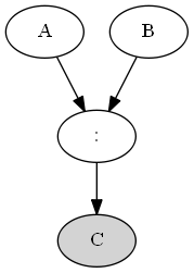
Type 3 (common effect OR v-structure)

Active Triplets

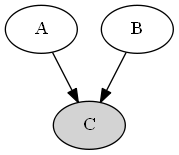
Given that \(C\) is involved, \(A\) & \(B\) become dependent (loose their absolute independence).

i.e.; \(P(A | B, C) eq P(A | C)\)

Also used for probabilistic reasoning called explain away effect.

Inactive Triplets (Absolute Independence)

Given that \(C\) is not involved, \(A\) & \(B\) are independent(Absolute Independence).

i.e.; \(P(A |B ) = P(A)\)

 

Type 4 (common effect on descendant OR v-structure with a bottom tail)

Type 4 is derived directly from Type 3.

Active Triplets

Given that \(C\) is involved, \(A\) and \(B\)  become dependent (loose their absolute independence).

i.e.; \(P(A | B, C) eq P(A | C)\)

 

Examples

Cancer example

Given

• \(P(C) = 0.01\)
• \(P(+ | C) = 0.9\)
• \(P(+ | !C) = 0.2\)

Directly Inferred

• \(P(!C) = 1 – P(C) = 1 – 0.01 = 0.99\)
• \(P(- | C) = 1 – P(+ | C) = 1 – 0.9 = 0.1\)
• \(P(- | !C) = 1 – P(+ | !C) = 1 – 0.2 = 0.8\)

 

Computations for Cancer Example

• \(P(+, C) = P(C) P(+ | C) = 0.01 * 0.9 = 0.009\)

 

 

• \(P(+, !C) = P(!C) P(+ | !C) = 0.99 * 0.2 = 0.198\)

 

 

• \(P(+) = P(+ | C) P(C) \hspace{1mm}+\hspace{1mm} P(+ | !C) P(!C)\)

\(\Rightarrow 0.9 * 0.01 \hspace{1mm}+\hspace{1mm} 0.2 * 0.99 = 0.207\)

 

 

• \(P(C | +) = \frac{P(C) P(+ | C)}{P(+)}\)

\(\Longrightarrow\) resolution: (Bayes’ Rule)

 

\(\Rightarrow \frac{P(C) P(+ | C)}{P(C) P(+ | C) \hspace{1mm}+\hspace{1mm} P(!C) P(+ | !C)}\)

 

\(\Rightarrow \frac{0.01 * 0.9 }{ 0.01 * 0.9 \hspace{1mm}+\hspace{1mm} 0.99 * 0.2} = 0.04347826087\)

 

 

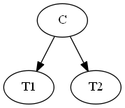
Two test Cancer example

Given

• \(P(C) = 0.01\)     \(\Longrightarrow P(!C) = 0.99\)
• \(P(+ | C) = 0.9\)      \(\Longrightarrow P(- | C) = 0.1\)
• \(P(+ | !C) = 0.2\)      \(\Longrightarrow P(- | !C) = 0.8\)

 

Computations for two test cancer example

• \(P(C | T1 = +, T2 = +) = P(C | +_1, +_2)\)

 

\(\Rightarrow \frac{P(+_1, +_2 | C) P(C)}{P(+_1, +_2 | C) P(C) \hspace{1mm}+\hspace{1mm} P(+_1, +_2 | !C) P(!C)}\)

 

\(\Rightarrow \frac{P(+_1 |+_2, C) P( +_2 | C) P(C)}{P(+_1 |+_2, C) P(+_2 | C) P(C) \hspace{1mm}+\hspace{1mm} P(+_1 |+_2, !C) P(+_2 | !C) P(!C)}\)

 

\(\Rightarrow \frac{P(+_1 | C) P(+_2 | C) P(C)}{P(+_1 | C) P(+_2 | C) P(C) \hspace{1mm}+\hspace{1mm} P(+_1 | !C) P(+_2 | !C) P(!C)}\)

\(\Longrightarrow\) resolution: \(P( +_1 | +_2, C) = P(+_1 | C)\) and \(P( +_1 | +_2, !C) = P(+_1 | !C)\) (Since C is the root of both \(+_1\) and \(+_2\), they become independent)

 

\(\Rightarrow \frac{0.9 * 0.9 * 0.01}{0.9 * 0.9 * 0.01 \hspace{1mm}+\hspace{1mm} 0.2 * 0.2 * 0.99} = 0.1698113208\)

 

 

• \(P(C | T1 = +, T2 = -) = P(C | +,-)\)

 

\(\Rightarrow \frac{P(+, – | C) P(C)}{P(+, – | C) P(C) \hspace{1mm}+\hspace{1mm} P(+, – | !C) P(!C)}\)

 

\(\Rightarrow \frac{P(+ |-, C) P( – | C) P(C)}{P(+ |-, C) P(- | C) P(C) \hspace{1mm}+\hspace{1mm} P(+ |-, !C) P(- | !C) P(!C)}\)

 

\(\Rightarrow \frac{P(+ | C) P(- | C) P(C)}{P(+ | C) P(- | C) P(C) \hspace{1mm}+\hspace{1mm} P(+ | !C) P(- | !C) P(!C)}\)

\(\Longrightarrow\) resolution: \(P( + | -, C) = P(+ | C)\) and \(P( + | -, !C) = P(+ | !C)\) (Since C is the root of both \(+\) and \(-\), they become independent)

 

\(\Rightarrow \frac{0.9 * 0.1 * 0.01}{0.9 * 0.1 * 0.01 \hspace{1mm}+\hspace{1mm} 0.2 * 0.8 * 0.99} = 0.00564971\)

 

 

• \(P(T2 = + | T1 = +) = P(+_2 | +_1)\)

 

\(\Rightarrow P(+_2 | +_1, C) P(C | +_1) \hspace{1mm}+\hspace{1mm} P(+_2 | +_1, !C) P(!C | +_1)\)

 

\(\Rightarrow P(+_2 | C) P(C | +_1) \hspace{1mm}+\hspace{1mm} P(+_2 | !C) P(!C | +_1)\)

\(\Longrightarrow\) resolution: \(P(+_2 | +_1, C) = P(+_2 | C)\) (since both \(+_1\) and \(+_2\) are conditionally independent in presence of \(C\))

 

\(\Rightarrow P(+_2 | C) \frac{P(C) P(+_1 | C)}{P(C) P(+_1 | C) \hspace{1mm}+\hspace{1mm} P(!C) P(+_1 | !C)} \hspace{1mm}+\hspace{1mm} P(+_2 | !C) \frac{P(!C) P(+_1 | !C)}{P(C) P(+_1 | C) \hspace{1mm}+\hspace{1mm} P(!C) P(+_1 | !C)}\)

 

\(\Rightarrow 0.9 * 0.04347826087 \hspace{1mm}+\hspace{1mm} 0.2 * 0.95652173913 = 0.23043478260\)

 

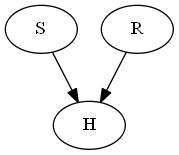
Example for Converged Conditionals on a Single node

Given

• \(P(S) = 0.7\)
• \(P(R) = 0.01\)
• \(P(H | S, R) = 1\)
• \(P( H | !S, R) = 0.9\)
• \(P(H | S, !R) = 0.7\)
• \(P(H | S, !R) = 0.7\)

 

Computations for converged conditionals on a single node

• \(P(R | S) = P(R) = 0.01\)

\(\Longrightarrow\) resolution: (Absolute Independence)

 

 

• \(P(R | H, S) = \frac{P(R) P(H, S | R)}{P(H,S)}\)

 

\(\Rightarrow \frac{P(R) P(H | S ,R) P(S | R)}{P(H | S)P(S)}\)

 

\(\Rightarrow \frac{P(R) P(H | S ,R) P(S)}{P(H | S) P(S)}\)

\(\Longrightarrow\) resolution: \(P(S | R) = P(S)\) (Since \(S\) and \(R\) are conditionally independent in absence of \(H\) (absolute independence) )

 

\(\Rightarrow \frac{P(R) P(H | S ,R)}{P(H | S)}\)

 

\(\Rightarrow \frac{P(R) P(H | S ,R)}{P(R) P(H | S, R) \hspace{1mm}+\hspace{1mm} P(!R) P(H | S, !R)}\)

 

\(\Rightarrow \frac{1 * 0.01}{1 * 0.01 \hspace{1mm}+\hspace{1mm} 0.7 * 0.99} = 0.01422475\)

 

 

• \(P(R | H) = \frac{P(R)P(H|R)}{P(H)}\)

 

\(\Rightarrow \frac{P(R)P(H|R)}{P(R)P(H|R) \hspace{1mm}+\hspace{1mm} P(!R)P(H|!R)}\)

 

\(\Rightarrow \frac{P(R)(\hspace{1mm}P(S)P(H|S,R)\hspace{1mm}+\hspace{1mm}P(!S)P(H|!S,R)\hspace{1mm})}{P(R)(\hspace{1mm}P(S)P(H|S,R)\hspace{1mm}+\hspace{1mm}P(!S)P(H|!S,R)\hspace{1mm}) \hspace{1mm}+\hspace{1mm} P(!R)(\hspace{1mm}P(S)P(H|S,!R)\hspace{1mm}+\hspace{1mm}P(!S)P(H|!S,!R)\hspace{1mm})}\)

 

\(\Rightarrow \frac{0.01 * 0.97}{0.01 * 0.97 + 0.99 * 0.52} = 0.01849380\)